RSA and How It Works

In the last post we discussed Euler’s theorem:

If $$a$$ and $$n$$ are relatively prime, then $$!a^{\phi(n)} \equiv 1 \pmod{n}$$ where $$\phi(n)$$ is the number of integers in $$[1,n]$$ that are relatively prime to $$n$$.

For any positive integer $$n = p_1^{k_1}p_2^{k_2}p_3^{k_3}…p_r^{k_r} $$, where $$p$$ and $$k$$ are from the factored form under the fundamental theorem of arithmetic. We have $$!\phi(n) = n\prod_{p|n}(1 – \frac{1}{p})$$

Let’s consider a simpler case, $$n = pq$$, where $$p$$ and $$q$$ are two distinct primes. For this special case, $$\phi(n) = (p-1)(q-1)$$. We simply verify it as follows:

Because $$p$$ and $$q$$ are primes, integers in $$[1,pq]$$ that are relatively prime to $$pq$$ must be multiple of $$p$$ or multiple of $$q$$. There are $$q$$ multiples of $$p$$ and $$p$$ multiples of $$q$$, and $$pq$$ is counted twice. Therefore $$!\phi(n) = pq -p – q + 1 = (p-1)(q-1)$$

RSA works as follows:

  • Two large different primes $$p$$ and $$q$$, and their product $$n = pq$$. When they are large, the factoring can be extremely hard.
  • An integer $$e$$ that satisfies $$\gcd(e, \phi(n)) = 1$$ is chosen. The pair $$(e, n)$$ are used as the public key and serve the purpose of encryption. $$! m’ = \mathrm{rem}(m^e, n)$$
  • An integer $$d$$ that satisfies $$de \equiv 1 \pmod{\phi(n)}$$ is chosen. The pair $$(d, n)$$ are used as the private key and serve the purpose of decryption. $$! m = \mathrm{rem}((m’)^d, n)$$

Let’s understand why the decryption works?

$$!\begin{align}
m’ & = \mathrm{rem}(m^e, n) \\
m’ & \equiv m^e \pmod{n} \\
(m’)^d & \equiv m^{ed} \pmod{n}
\end{align}$$

We know $$de \equiv 1 \pmod{\phi(n)}$$, so $$\exists~r \in \mathbb{Z}$$, such that $$r\phi(n) + 1 = de$$. We substitute it back to the one above,

$$!\begin{align}
(m’)^d & \equiv m^{r\phi(n) + 1} \pmod{n}\\
& \equiv (m^{\phi(n)})^rm  \pmod{n} \\
& \equiv m \pmod{n}
\end{align}$$

Now we can see that $$! m  = \mathrm{rem}((m’)^d, n)$$

Implementation wise, there are are few things to note:

  • We know $$n = pq$$, so as long as both $$p$$ and $$q$$ don’t divide $$m$$, we have $$\gcd(m,n) = 1$$. When $$p$$ and $$q$$ are large, this is usually the case. However, if $$\gcd(m,n) \neq 1$$, the whole system will break.
Finding Greatest Common Divisor of Two Integers Using Pulverizer

Pulverizer is a method similar to Euclead’s algorithm that finds the greatest common divisor (GCD) of two integers. It logs the calculations so that how such GCD can be achieved with linear combination of the two integers is also found.

Here is a simple example in C:

int pulverizer(long a, long b){
    long xa[] = {1,0};
    long xb[] = {0,1};
    
    while(a != b){
        if(a > b){
            a = a - b;
            xa[0] = xa[0] - xb[0];
            xa[1] = xa[1] - xb[1];
        }else{
            b = b - a;
            xb[0] = xb[0] - xa[0];
            xb[1] = xb[1] - xa[1];
        }
    }
    
    printf("GCD(a,b) = %ld; coefficients can be (%ld, %ld) or (%ld, %ld).\n", a, xa[0], xa[1], xb[0], xb[1]);
}

Pulverizer is very useful in finding the multiplicative inverse of an integer $$k$$ modulo a relatively prime number $$p$$. Consider the following:$$!\gcd(k,p) = 1$$ There exists a pair of integers $$(s,t)$$ such that $$!sp + tk = 1$$

Therefore, $$1-tk = sp \implies p | 1-tk \implies tk \equiv 1 \pmod{p}$$.

Alternatively, Fermat’s little theorem and its generalization, Euler’s theorem, can also be used to find the multiplicative inverse.

Proof of Euler’s Theorem without Advanced Techniques

Euler’s Theorem

If $$a$$ and $$n$$ are relatively prime, then $$!a^{\phi(n)} \equiv 1 \pmod{n}$$ where $$\phi(n)$$ is the number of integers in $$[1,n]$$ that are relatively prime to $$n$$.

The Euler’s Totient Function

Single Prime

First, we examine function $$\phi(p^k)$$, where $$p$$ is a prime:

In $$\{1,2,3,…,p^k\}$$,  the only integers that are not relatively prime to $$p^k$$ are the multiples of $$p$$, and there are $$\frac{p^k}{p} $$ of them. Therefore $$!\begin{align}\phi(p^k) &= p^k – \frac{p^k}{p} \\ &= p^k (1- \frac{1}{p})\end{align}$$

Multiplicative Function

Lemma: if $$a$$ and $$b$$ are relatively prime, then $$\phi(ab) = \phi(a)\phi(b)$$

Proof:

We first arrange the numbers $$\{1,2,3,…,ab\}$$ by rows to a $$b \times a$$ matrix:

$$!\begin{bmatrix} 1 & 2 &  \dots & a \\
a+1 & a+ 2&  \dots & 2a\\
2a+ 1 & 2a+ 2 &  \dots & 3a\\
\vdots & \vdots & \ddots & \vdots\\
(b-1)a + 1 & (b-1)a +2 &\dots &  ab
\end{bmatrix}$$

This way, numbers in the same column are congruent to each other modulo $$a$$. Specifically, the element $$u_{ij}$$ at row i has the following property:

$$!\mathrm{rem}(u_{ij}, a) = j$$

We know (same as Euclid’s algorithm) that, $$!\gcd(u_{ij},a) = \gcd(\mathrm{rem}(u_{ij}, a), a) = \gcd(j,a)$$

This is to say that, if $$j \in \{1,2,3,…,a\}$$ satisfies $$\gcd(j,a) = 1$$, all the numbers in column $$j$$ are relatively prime to $$a$$, and there are $$\phi(a)$$ such columns in total.

Now let’s examine a column. The numbers in column $$j$$ can be written as: $$!\begin{bmatrix}
j\\
j+a\\
j+2a\\
\vdots\\
j+(b-1)a
\end{bmatrix}$$

Corollary: the remainders of the numbers in a column modulo b form a permutation of the sequence $$\{0,1,2,3,…,b-1\}$$.

This is equivalent to that each of the $$b$$ numbers in the row has a different remainder modulo b.We can prove it by contradiction:

Suppose $$!j+sa \equiv j+ta \pmod{b}$$ where $$b-1 \geq s > t \geq 0$$, we have $$!sa \equiv ta \pmod{b}$$ $$!(s-t)a \equiv 0 \pmod{b}$$

We know that $$\gcd(a,b) = 1$$, and (s-t) must be smaller than $$b$$, so there is contradiction.

Now, this corollary shows that every column has $$\phi(b)$$ numbers that are relatively prime to $$b$$.

Number $$u_ij$$ is relatively prime to $$ab$$ if and only if it is relatively to both $$a$$ and $$b$$. In other words, it must be on one of the $$\phi(a)$$ columns described above, and in one of the $$\phi(b)$$ positions on that column. Therefore, $$!\phi(ab) = \phi(a)\phi(b)$$

This can be applied to any positive integer $$n = p_1^{k_1}p_2^{k_2}p_3^{k_3}…p_r^{k_r} $$, where $$p$$ and $$k$$ are from the factored form under the fundamental theorem of arithmetic. We have $$!\phi(n) = n\prod_{p|n}(1 – \frac{1}{p})$$

Proof of the Theorem

We’ve finally come to prove that $$a^{\phi(n)} \equiv 1 \pmod{n}$$.

Lemma: Let $$m_1,m_2,m_3,…,m_{\phi(n)} $$ be the $$\phi(n)$$ integers that are relatively prime to n and in the range of $$[1, n]$$. Then there will no two of them, such that $$am_j \equiv am_i \pmod{n}$$, and all the remainders $$\mathrm{rem}(am_1, n), \mathrm{rem}(am_2, n), \mathrm{rem}(am_3, n), …, \mathrm{rem}(am_\phi(n), n)$$ form a permutation of the sequence $$\{m_1,m_2,m_3,…,m_{\phi(n)} \}$$.

Proof by contradiction:

Assume there is a pair of $$i$$ and $$j$$, such that $$am_j \equiv am_i \pmod{n}$$. Then $$a (m_j – m_i) \equiv 0 \pmod{n}$$. Since $$\gcd(a,n) = 0$$, $$m_j – m_i $$ must be divisible by $$n$$, which leads to contradiction. So we proved the difference between any $$am_i$$ and $$am_j$$. Also, $$\gcd(\mathrm{rem}(am, n), n) = gcd(am, n) = 1$$. Therefore, by definition, $$\mathrm{rem}(am, n) \in \{m_1,m_2,m_3,…,m_{\phi(n)} \}$$.

With this lemma, we can compute the congruence of the product of $$m_1,m_2,m_3,…,m_{\phi(n)}$$:

$$!\begin{align}
\prod_{i=1}^{\phi(n)}am_i & = a^{\phi(n)}\prod_{i=1}^{\phi(n)}\\
a^{\phi(n)}\prod_{i=1}^{\phi(n)}m_i & \equiv \prod_{i=1}^{\phi(n)}m_i \pmod{n}
\end{align}$$

For simplicity, we assign $$M = \prod_{i=1}^{\phi(n)}m_i$$, so we have $$!(a^{\phi(n)} – 1) M \equiv 0 \pmod{n}$$

Because $$M$$ is relatively prime to $$n$$, $$a^{\phi(n)} – 1$$ must be divisible by $$n$$.

Done.

Getting Good Performance with VMware Workstation Player

VMware Workstation Player has always been my favorite solution for desktop virtualization. It’s free, well-featured and easy to use. The main issue with it is the performance, especially the anomalously high disk utilization. Installing a guest system on a SSD is not always possible and affordable, and the excessive access may cause unwanted waste on the limited lifetime of the SSD.

Anyway, it accesses the disk frequently for reasons. Only a few years ago, many PCs were running with 512 MB of RAM. It was hard to allocate adequate memory for a guest system so there were many techniques developed to make the virtualization possible. Basically, they are the equivalences of virtual memory or SWAP.

However, things are much different now, where modern PCs are easily 8, 16 or even 32 GB of memory (the price is currently insane though LOL). I am using a laptop with 12 GB RAM, so allocating 4 GB of memory is usually sufficient for most of guest operating systems and at the same time should not create any significant negative impact to the host system. The following three tweaks should prevent the unnecessary disk access.

First, disable the virtual memory or swap in guest system. This is very optional because an operating system usually has highly optimized strategies of how to use virtual memory or swap. As long as you don’t open too may programs or pages, the systems will stick to physical memory. Disabling virtual memory restricts the flexibility. However, if you are very annoyed the noise of disks like me, you can turn it off.

Second, disable Memory Trimming. Memory Trimming is helpful when the overall RAM is low. It shrinks the guest RAM by storing inactive chunks of memory to the hard disk when the host needs more memory. In other words, it’s the host-managed virtual memory for a guest system. It can be disabled by adding the following line in the virtual machine configuration file (.vmx):

MemTrimRate= "0" 

Finally and most importantly, disable the virtual machine paging file (uuid.vmem). If you only want to use the guest system like a normal computer, and you have no need for crash recovering or creating snapshots (you don’t have snapshots in Player anyways), then there is no need to have a copy of the guest RAM in you disk. Disabling the file will make your life so much better. Just add the following line in the configuration file:

mainMem.useNamedFile = "false"

Now, your guest system only accesses your disk when it actually accesses its own disk. For any PC with sufficient RAM, the performance increase is very obvious.

References:
http://sanbarrow.com/vmx/vmx-advanced.html#mainmem
https://pubs.vmware.com/workstation-9/index.jsp?topic=%2Fcom.vmware.ws.using.doc%2FGUID-A968EF50-BA25-450A-9D1F-F8A9DEE640E7.html

Enable NVIDIA Optimus on Linux Deepin

Of course there is no real NVIDIA Optimus on Linux, but I found an article that gives some workaround: https://bbs.deepin.org/forum.php?mod=viewthread&tid=132312. Below are the steps described in the article.

Install drivers

sudo apt-get install bumblebee-nvidia nvidia-driver nvidia-settings

Verify the installation

sudo apt-get install mesa-utils

note: mesa-utils package provides useful tools to show glx information

optrun glxinfo | grep NVIDIA

note: this step checks whether the installation succeeded.

optirun glxgears -info

note: if you see a notice of your graphics card, you are good.

Run games with your nvidia graphics

Primusrun game

or

optirun game

to run steam games:

https://support.steampowered.com/kb_article.php?ref=6316-GJKC-7437

Windows 10 update KB3201845 causes disk usage issue

2 days ago, my girlfriend was playing World of Warcraft on my desktop computer which had just applied a new Windows 10 update, and she told me my computer was super laggy, and after restarted the computer a few times it did not get any better. So I took a look.

Process System was apparently accessing my disk like no tomorrow. Then I opened Resource Monitor to find out what files was it really working with. And it turned out to be something I had never seen:

C:\Windows\Temp\WPR_initiated_DiagTrackAotLogger_WPR System Collector.etl

And what is WPR exactly? After some search on Google, I found that it stands for Windows Performance Recorder, and its purpose , as it claims, is to track the performance and the resources consumption of a computer. Such thing should be used to help improve the performance, but funny enough, it made my computer barely usable. (link)

I kept searching, and finally I found temporary solution, but a solution nonetheless. (link)

wpr -cancel

I wrapped it into a .bat file, and told my girlfriend to execute it as admin should it happen again.

Things weren’t done yet. Yesterday my laptop received windows update as well, the same issue appeared. So I have become certain that something in this update was awfully wrong. Although thanks to the SSD, my laptop was still quite responsive, this shall not be tolerated. And I searched on Google again, and this time, I noticed many more users are suffering from the same issue than I did it the first time. And under the post I found the temporary solution, I found the ultimate fix (hopefully):

Go to All settings -> Privacy -> Feedback & diagnostics
change “Send your data to Microsoft” to Basic/Enhanced

I noticed significant change with my disk usage when I switched to Basic.


Fix for “internal error” connecting with RDP

The windows remote desktop has stopped working for me for a couple of days, and at the same time FIFA 17 was not launching either, but crashing at the language select screen. I never thought they’d be the same issue, until I fixed one and the other was also magically fixed!

The symptom was that, when clicking “connect”, the following error message popped up “An internal error occurred.”. Sometimes instead of the error message, it stuck at “initiating remote desktop connection”. Then I launched Ubuntu in a virtual machine, and I could connect to the remote desktop using a client in Ubuntu. Another thing I noticed is that, on my Windows, when I chose to connect to a target that did not exist, it still got the same error or simply stuck. This means two things:

  1. The remote server is working
  2. The connection is working

So I started to look on the internet and eventually I found this fix:

netsh winsock reset all

http://superuser.com/a/984351/671434

Now everything is working. Cheers!

Learning from Data 4: Error and Noise

Learning from Data is a Machine Learning MOOC taught by Caltech Professor Yaser Abu-Mostafa. I took the course in 2014 through edX. It was a great course, well-organized and into the details.

Recently I have been reviewing the notes and the summary of the course, and I thought I might just post them here. All my code used for the homework can be found at https://github.com/Chaoping/Learning-From-Data.

Lecture 4: Error and Noise

What is error? We wish to learn a hypothesis that approximates the target function, “$$h \approx f$$”. The error basically reflects how a hypothesis does the job. And we call it: “$$E(h,f)$$”. Then the pointwise error for any point can be defined as: $$!\mathrm{e}(h(\mathbf{x}), f(\mathbf{x}))$$

If we consider the overall $$E(h,f)$$ error as the average of the pointwise error, we have:

in-sample error: $$!E_{in}(h) = \frac{1}{N}\sum_{n=1}^{N}{\mathrm{e}(h(\mathbf{x}_n), f(\mathbf{x}_n))}$$

out-of-sample error: $$!E_{out}(h) = \mathbb{E}_\mathbf{x}[\mathrm{e}(h(\mathbf{x}), f(\mathbf{x}))]$$

But how do we measure the error? The error measure should be specified by the user. However such thing isn’t always possible. So often we take alternatives that are:

  • Plausible, meaning the measure makes sense or at least intuitively correct. For example the squared error is equivalent to Gaussian noise.
  • Friendly, meaning it is convex so that the learning algorithm can work effectively, or it may even have a closed-form solution just like the squared error.

With the error measure defined, we then can have a learning algorithm to pick $$g$$ out of $$H$$.

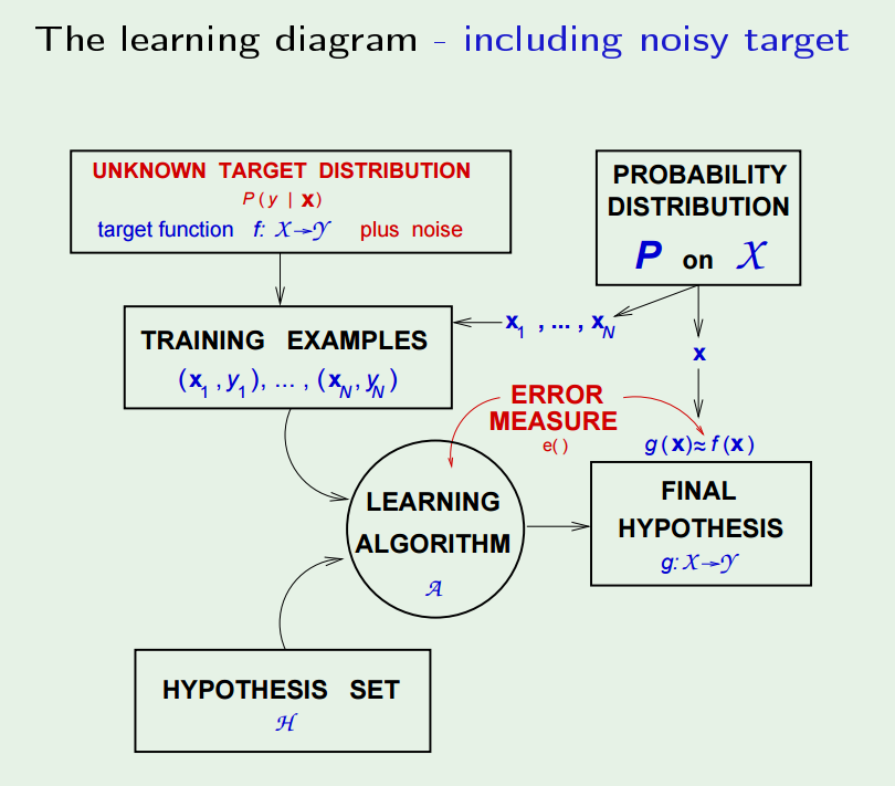
Now, let’s reconsider about target function – is it really a function? No, because very possible that two identical input may have different output. So instead, we have a “target distribution”: $$!P(y|\mathbf{x})$$ Each point is generated from the joint distribution of $$!P(\mathbf{x})P(y|\mathbf{x})$$

And the “noisy target” can be seen as a combination of a deterministic target: $$!f(\mathbf{x}) = \mathbb{E}(y|\mathbf{x})$$ plus the noise: $$!y-f(\mathbf{x})$$

Finally, the learning diagram shall look like this:

the_learning_diagram_including_noisy_target

At this point, we know:

Learning is feasible. It is likely that $$!E_{in}(g) \approx E_{out}(g)$$

What we are trying to achieve is that $$g \approx f$$, or equivalently $$!E_{out}(g) \approx 0$$

So learning is split into 2 goals that have to be achieved at the same time:

  • $$E_{in}(g)$$ must be close to $$E_{out}(g)$$.
  • $$E_{in}(g)$$ must be small enough.

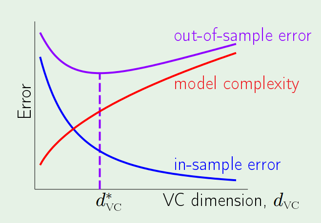
This leads to the following topics, where the model complexity will play a big role affecting both. The trade-off lies that the more complex a model is, the smaller $$E_{in}(g)$$ will be and at the same time it loses its ability to track $$E_{out}(g)$$.

sample_complexity_tradeoff


Learning from Data 3: The Linear Model I

Learning from Data is a Machine Learning MOOC taught by Caltech Professor Yaser Abu-Mostafa. I took the course in 2014 through edX. It was a great course, well-organized and into the details.

Recently I have been reviewing the notes and the summary of the course, and I thought I might just post them here. All my code used for the homework can be found at https://github.com/Chaoping/Learning-From-Data.

Lecture 3: The Linear Model I

First the Input Representation is discussed. Consider digit recognition of a grey-scale image of 16*16 pixels. The raw input would have 256+1 weights. However we know that something can be extract from the input, something more meaningful. For example the symmetry and the intensity. Now the raw inputs are transformed into features, and the number of features is much smaller than that of inputs.

Linear Regression is the most fundamental model to output real-value:$$!h(x) = \sum_{i=0}^{d}{w_ix_i} = \mathbf{w}^\intercal\mathbf{x}$$

To measure how a Linear Regression hypothesis $$h(x) = \mathbf{w}^\intercal\mathbf{x}$$ approximates the target function $$f(x)$$, we use squared error: $$(h(x) – f(x))^2$$. So the in sample error is: $$!E_{in}(h)=\frac{1}{N} \sum_{n=1}^{N}{(h(x_n)-y_n)^2}$$

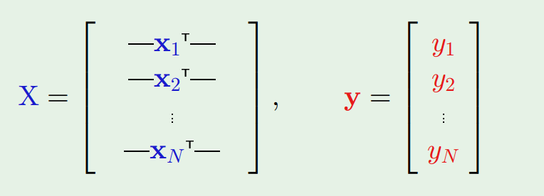
or equivalently, $$!E_{in}(\mathbf{w})=\frac{1}{N}||\mathbf{Xw} – \mathbf{y}||^2$$

where $$\mathbf{x}$$ and $$\mathbf{y}$$ are constructed as:

constructxandy

$$\mathbf{X}$$ and $$\mathbf{y}$$ are all constant as they are given from the sample, so we are minimizing $$E_{in}$$ in respect of $$\mathbf{w}$$. Since this is quadratic for $$\mathbf{w}$$, the minimum is achieved when $$!\nabla E_{in}(\mathbf{w})=\frac{2}{N}\mathbf{X}^\intercal(\mathbf{Xw} – \mathbf{y})=\mathbf{0}$$

$$!\mathbf{X}^\intercal\mathbf{X}\mathbf{w} = \mathbf{X}^\intercal\mathbf{y}$$

$$!\mathbf{w} = (\mathbf{X}^\intercal\mathbf{X})^{-1}\mathbf{X}^\intercal\mathbf{y}$$

$$\mathbf{X}^\dagger = (\mathbf{X}^\intercal\mathbf{X})^{-1}\mathbf{X}^\intercal$$ (pronounced as “x dagger”) is called the “pseudo-inverse of $$\mathbf{X}$$”. It has a very interesting property that $$\mathbf{X}^\dagger\mathbf{X}=\mathbf{I}$$

With the help of pseudo-inverse, learning the weights $$\mathbf{w}$$ becomes one-step, and it is very computation efficient even with a big sample set, because it shrinks the matrix to dimensions of the number of the weights, which usually is quite small compared to that of the sample size.

Binary outputs are also real-value outputs, at least a kind of, so that it is possible to use Linear Regression to work on classifications. It will work but it may not perform so well because instead of finding a boundary, it tries to minimize the squared distances. However, it would still be a very useful tool to setup the initial weights for a pocketed perceptron.

The last part of the lecture discussed non-linear transformation. In other words, the features can be the linear transformation of the original features, for example $$!(x_1, x_2) \to(x_1^2,x_2^2)$$. This will work because of the linearity in the weights.