Machine Learning – Chaoping Guo

Learning from Data 4: Error and Noise

Learning from Data is a Machine Learning MOOC taught by Caltech Professor Yaser Abu-Mostafa. I took the course in 2014 through edX. It was a great course, well-organized and into the details.

Recently I have been reviewing the notes and the summary of the course, and I thought I might just post them here. All my code used for the homework can be found at https://github.com/Chaoping/Learning-From-Data.

Lecture 4: Error and Noise

What is error? We wish to learn a hypothesis that approximates the target function, “$$h \approx f$$”. The error basically reflects how a hypothesis does the job. And we call it: “$$E(h,f)$$”. Then the pointwise error for any point can be defined as: $$!\mathrm{e}(h(\mathbf{x}), f(\mathbf{x}))$$

If we consider the overall $$E(h,f)$$ error as the average of the pointwise error, we have:

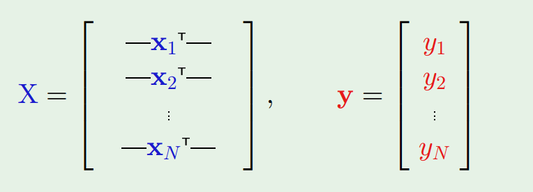
in-sample error: $$!E_{in}(h) = \frac{1}{N}\sum_{n=1}^{N}{\mathrm{e}(h(\mathbf{x}_n), f(\mathbf{x}_n))}$$

out-of-sample error: $$!E_{out}(h) = \mathbb{E}_\mathbf{x}[\mathrm{e}(h(\mathbf{x}), f(\mathbf{x}))]$$

But how do we measure the error? The error measure should be specified by the user. However such thing isn’t always possible. So often we take alternatives that are:

Plausible, meaning the measure makes sense or at least intuitively correct. For example the squared error is equivalent to Gaussian noise.
Friendly, meaning it is convex so that the learning algorithm can work effectively, or it may even have a closed-form solution just like the squared error.

With the error measure defined, we then can have a learning algorithm to pick $$g$$ out of $$H$$.

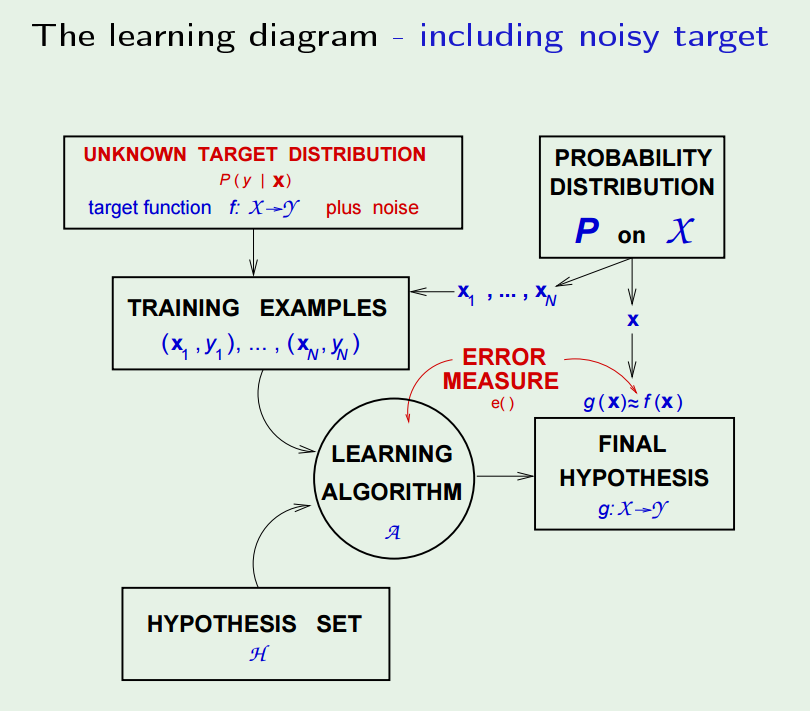
Now, let’s reconsider about target function – is it really a function? No, because very possible that two identical input may have different output. So instead, we have a “target distribution”: $$!P(y|\mathbf{x})$$ Each point is generated from the joint distribution of $$!P(\mathbf{x})P(y|\mathbf{x})$$

And the “noisy target” can be seen as a combination of a deterministic target: $$!f(\mathbf{x}) = \mathbb{E}(y|\mathbf{x})$$ plus the noise: $$!y-f(\mathbf{x})$$

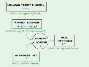
Finally, the learning diagram shall look like this:

At this point, we know:

Learning is feasible. It is likely that $$!E_{in}(g) \approx E_{out}(g)$$

What we are trying to achieve is that $$g \approx f$$, or equivalently $$!E_{out}(g) \approx 0$$

So learning is split into 2 goals that have to be achieved at the same time:

$$E_{in}(g)$$ must be close to $$E_{out}(g)$$.
$$E_{in}(g)$$ must be small enough.

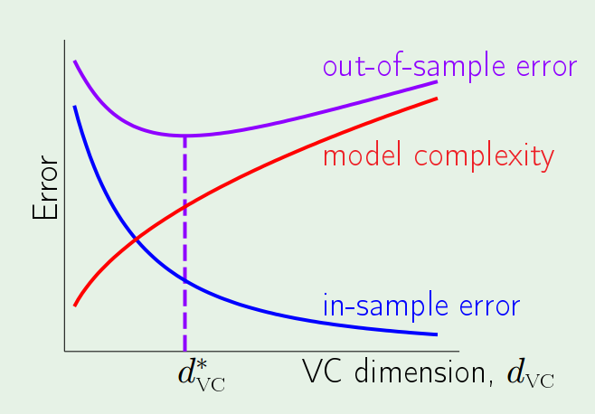
This leads to the following topics, where the model complexity will play a big role affecting both. The trade-off lies that the more complex a model is, the smaller $$E_{in}(g)$$ will be and at the same time it loses its ability to track $$E_{out}(g)$$.

Learning from Data 3: The Linear Model I

Learning from Data is a Machine Learning MOOC taught by Caltech Professor Yaser Abu-Mostafa. I took the course in 2014 through edX. It was a great course, well-organized and into the details.

Lecture 3: The Linear Model I

First the Input Representation is discussed. Consider digit recognition of a grey-scale image of 16*16 pixels. The raw input would have 256+1 weights. However we know that something can be extract from the input, something more meaningful. For example the symmetry and the intensity. Now the raw inputs are transformed into features, and the number of features is much smaller than that of inputs.

Linear Regression is the most fundamental model to output real-value:$$!h(x) = \sum_{i=0}^{d}{w_ix_i} = \mathbf{w}^\intercal\mathbf{x}$$

To measure how a Linear Regression hypothesis $$h(x) = \mathbf{w}^\intercal\mathbf{x}$$ approximates the target function $$f(x)$$, we use squared error: $$(h(x) – f(x))^2$$. So the in sample error is: $$!E_{in}(h)=\frac{1}{N} \sum_{n=1}^{N}{(h(x_n)-y_n)^2}$$

or equivalently, $$!E_{in}(\mathbf{w})=\frac{1}{N}||\mathbf{Xw} – \mathbf{y}||^2$$

where $$\mathbf{x}$$ and $$\mathbf{y}$$ are constructed as:

$$\mathbf{X}$$ and $$\mathbf{y}$$ are all constant as they are given from the sample, so we are minimizing $$E_{in}$$ in respect of $$\mathbf{w}$$. Since this is quadratic for $$\mathbf{w}$$, the minimum is achieved when $$!\nabla E_{in}(\mathbf{w})=\frac{2}{N}\mathbf{X}^\intercal(\mathbf{Xw} – \mathbf{y})=\mathbf{0}$$

$$!\mathbf{X}^\intercal\mathbf{X}\mathbf{w} = \mathbf{X}^\intercal\mathbf{y}$$

$$!\mathbf{w} = (\mathbf{X}^\intercal\mathbf{X})^{-1}\mathbf{X}^\intercal\mathbf{y}$$

$$\mathbf{X}^\dagger = (\mathbf{X}^\intercal\mathbf{X})^{-1}\mathbf{X}^\intercal$$ (pronounced as “x dagger”) is called the “pseudo-inverse of $$\mathbf{X}$$”. It has a very interesting property that $$\mathbf{X}^\dagger\mathbf{X}=\mathbf{I}$$

With the help of pseudo-inverse, learning the weights $$\mathbf{w}$$ becomes one-step, and it is very computation efficient even with a big sample set, because it shrinks the matrix to dimensions of the number of the weights, which usually is quite small compared to that of the sample size.

Binary outputs are also real-value outputs, at least a kind of, so that it is possible to use Linear Regression to work on classifications. It will work but it may not perform so well because instead of finding a boundary, it tries to minimize the squared distances. However, it would still be a very useful tool to setup the initial weights for a pocketed perceptron.

The last part of the lecture discussed non-linear transformation. In other words, the features can be the linear transformation of the original features, for example $$!(x_1, x_2) \to(x_1^2,x_2^2)$$. This will work because of the linearity in the weights.

Learning from Data 2: Is Learning Feasible?

Learning from Data is a Machine Learning MOOC taught by Caltech Professor Yaser Abu-Mostafa. I took the course in 2014 through edX. It was a great course, well-organized and into the details.

Lecture 2: Is Learning Feasible?

Lecture 2 starts with a question of probability: Can a sample tell anything about the population? In probability, the answer is yes – and we know the bigger the sample, the better it represents the population. Now instead of confidence interval, here we use another way to measure the sample size – precision trade off, that is, the Hoeffding’s inequality: $$!\mathbb{P}[|\mu – \nu |>\epsilon] \le 2e^{-2\epsilon^2N}$$

With Hoeffding’s Inequality, we can say that “$$\mu = \nu$$” is “P.A.C” true (probably, approximately, correct). “Probably” because the probability of violation is small, and “approximately” because $$\epsilon$$ is small (with good size of $$N$$).

Now, consider a learning problem, the only assumption is that, the data we have, is simply a sample, generated with a probability distribution. The analogy is that, we know how a hypothesis performs on the training set, and with Hoeffding’s Inequality we believe it should reflect how the hypothesis will work on the data we haven’t seen. By changing the notation of $$\mu$$ and $$\nu$$, we have $$!\mathbb{P}[|E_\mathrm{in}(h) – E_\mathrm{out}(h) |>\epsilon] \le 2e^{-2\epsilon^2N}$$

However there is yet another problem – Hoeffding’s Inequality applies to each one of the hypothesis, but when we combine many hypotheses all together, it fails. It is because we “tried too hard”.

To solve it, we can give it a union bound. Since the final hypothesis $$g$$ is one element in the hypothesis set $$H$$, without giving any extra assumptions, we can safely say that $$!\mathbb{P}[|E_\mathrm{in}(g) – E_\mathrm{out}(g) |>\epsilon] \le 2Me^{-2\epsilon^2N}$$

Now with $$M$$ being the number of hypotheses in $$H$$, we once again give it a bound.

Learning from Data 1: The Learning Problem

Learning from Data is a Machine Learning MOOC taught by Caltech Professor Yaser Abu-Mostafa. I took the course in 2014 through edX. It was a great course, well-organized and into the details.

Lecture 1: The Learning Problem

Lecture 1 is the brief introduction of the course. It answered the question of “what is learning”. So the essence of learning is that:

A pattern exists, which we are trying to find
We cannot pin it down mathematically (otherwise we would not need to “learn”)
We have data

And a learning problem can be formalized as:

Input: $$\mathbf{x}$$
Output: $$y$$
Target function: $$f: X \rightarrow Y$$, which we do not know
Data: $$(\mathbf{x}_1, y_1), (\mathbf{x}_2,y_2),…,(\mathbf{x}_N,y_N)$$ $$!\downarrow$$
Hypothesis: $$g: X \rightarrow Y$$, to approximate the target function.

In fact, to come up with the final hypothesis $$g$$, we are using a hypothesis set $$H$$, in which there are infinite hypotheses. A chart in the course slides shows the concept:

The Hypothesis Set $$H$$ and the Learning Algorithm $$A$$ together are referred as the “learning model”.

Then the simplest example of learning is the “perceptron”, its linear formula $$h \in H$$ can be written as: $$! h(x) = \mathrm{sign} ((\sum_{i=1}^{d}{w_i}{x_i})-t)$$ where t represents the threshold.

If we change the notation of $$t$$ to $$w_0$$, and introduce an artificial coordinate $$x_0 = 1$$, all of a sudden it can now be written as: $$!h(x) = \mathrm{sign}(\sum_{i=0}^{d}{w_i}{x_i})$$ or equivalently, $$!h(x) = \mathrm{sign}(\mathbf{w}^\intercal\mathbf{x})$$

The concept of perceptron’s learning algorithm is rather intuitive, that it tries to correct a random misclassified point every iteration, by: $$!\mathbf{w} = \mathbf{w} + {y_n}\mathbf{x_n}$$ The correction can be visualized as the following:

The algorithm keeps iterating, and eventually it will come to a point where all points are correctly classified, so long as the data is linearly-separable.

There are 3 types of learning:

Supervised Learning: input, output
Unsupervised Learning: input, no output
Reinforcement Learning: input, grade for output