Learning from Data is a Machine Learning MOOC taught by Caltech Professor Yaser Abu-Mostafa. I took the course in 2014 through edX. It was a great course, well-organized and into the details.
Recently I have been reviewing the notes and the summary of the course, and I thought I might just post them here. All my code used for the homework can be found at https://github.com/Chaoping/Learning-From-Data.
Lecture 3: The Linear Model I
First the Input Representation is discussed. Consider digit recognition of a grey-scale image of 16*16 pixels. The raw input would have 256+1 weights. However we know that something can be extract from the input, something more meaningful. For example the symmetry and the intensity. Now the raw inputs are transformed into features, and the number of features is much smaller than that of inputs.
Linear Regression is the most fundamental model to output real-value:$$!h(x) = \sum_{i=0}^{d}{w_ix_i} = \mathbf{w}^\intercal\mathbf{x}$$
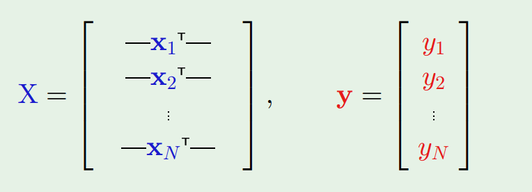
To measure how a Linear Regression hypothesis $$h(x) = \mathbf{w}^\intercal\mathbf{x}$$ approximates the target function $$f(x)$$, we use squared error: $$(h(x) – f(x))^2$$. So the in sample error is: $$!E_{in}(h)=\frac{1}{N} \sum_{n=1}^{N}{(h(x_n)-y_n)^2}$$
or equivalently, $$!E_{in}(\mathbf{w})=\frac{1}{N}||\mathbf{Xw} – \mathbf{y}||^2$$
where $$\mathbf{x}$$ and $$\mathbf{y}$$ are constructed as:
$$\mathbf{X}$$ and $$\mathbf{y}$$ are all constant as they are given from the sample, so we are minimizing $$E_{in}$$ in respect of $$\mathbf{w}$$. Since this is quadratic for $$\mathbf{w}$$, the minimum is achieved when $$!\nabla E_{in}(\mathbf{w})=\frac{2}{N}\mathbf{X}^\intercal(\mathbf{Xw} – \mathbf{y})=\mathbf{0}$$
$$!\mathbf{X}^\intercal\mathbf{X}\mathbf{w} = \mathbf{X}^\intercal\mathbf{y}$$
$$!\mathbf{w} = (\mathbf{X}^\intercal\mathbf{X})^{-1}\mathbf{X}^\intercal\mathbf{y}$$
$$\mathbf{X}^\dagger = (\mathbf{X}^\intercal\mathbf{X})^{-1}\mathbf{X}^\intercal$$ (pronounced as “x dagger”) is called the “pseudo-inverse of $$\mathbf{X}$$”. It has a very interesting property that $$\mathbf{X}^\dagger\mathbf{X}=\mathbf{I}$$
With the help of pseudo-inverse, learning the weights $$\mathbf{w}$$ becomes one-step, and it is very computation efficient even with a big sample set, because it shrinks the matrix to dimensions of the number of the weights, which usually is quite small compared to that of the sample size.
Binary outputs are also real-value outputs, at least a kind of, so that it is possible to use Linear Regression to work on classifications. It will work but it may not perform so well because instead of finding a boundary, it tries to minimize the squared distances. However, it would still be a very useful tool to setup the initial weights for a pocketed perceptron.
The last part of the lecture discussed non-linear transformation. In other words, the features can be the linear transformation of the original features, for example $$!(x_1, x_2) \to(x_1^2,x_2^2)$$. This will work because of the linearity in the weights.