Learning from Data is a Machine Learning MOOC taught by Caltech Professor Yaser Abu-Mostafa. I took the course in 2014 through edX. It was a great course, well-organized and into the details.
Recently I have been reviewing the notes and the summary of the course, and I thought I might just post them here. All my code used for the homework can be found at https://github.com/Chaoping/Learning-From-Data.
Lecture 1: The Learning Problem
Lecture 1 is the brief introduction of the course. It answered the question of “what is learning”. So the essence of learning is that:
- A pattern exists, which we are trying to find
- We cannot pin it down mathematically (otherwise we would not need to “learn”)
- We have data
And a learning problem can be formalized as:
- Input: $$\mathbf{x}$$
- Output: $$y$$
- Target function: $$f: X \rightarrow Y$$, which we do not know
- Data: $$(\mathbf{x}_1, y_1), (\mathbf{x}_2,y_2),…,(\mathbf{x}_N,y_N)$$ $$!\downarrow$$
- Hypothesis: $$g: X \rightarrow Y$$, to approximate the target function.
In fact, to come up with the final hypothesis $$g$$, we are using a hypothesis set $$H$$, in which there are infinite hypotheses. A chart in the course slides shows the concept:
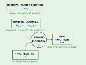
The Hypothesis Set $$H$$ and the Learning Algorithm $$A$$ together are referred as the “learning model”.
Then the simplest example of learning is the “perceptron”, its linear formula $$h \in H$$ can be written as: $$! h(x) = \mathrm{sign} ((\sum_{i=1}^{d}{w_i}{x_i})-t)$$ where t represents the threshold.
If we change the notation of $$t$$ to $$w_0$$, and introduce an artificial coordinate $$x_0 = 1$$, all of a sudden it can now be written as: $$!h(x) = \mathrm{sign}(\sum_{i=0}^{d}{w_i}{x_i})$$ or equivalently, $$!h(x) = \mathrm{sign}(\mathbf{w}^\intercal\mathbf{x})$$
The concept of perceptron’s learning algorithm is rather intuitive, that it tries to correct a random misclassified point every iteration, by: $$!\mathbf{w} = \mathbf{w} + {y_n}\mathbf{x_n}$$ The correction can be visualized as the following:
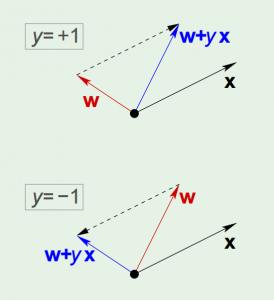
The algorithm keeps iterating, and eventually it will come to a point where all points are correctly classified, so long as the data is linearly-separable.
There are 3 types of learning:
- Supervised Learning: input, output
- Unsupervised Learning: input, no output
- Reinforcement Learning: input, grade for output