Author: Chaoping Guo

Learning from Data is a Machine Learning MOOC taught by Caltech Professor Yaser Abu-Mostafa. I took the course in 2014 through edX. It was a great course, well-organized and into the details.

Recently I have been reviewing the notes and the summary of the course, and I thought I might just post them here. All my code used for the homework can be found at https://github.com/Chaoping/Learning-From-Data.

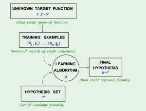
Lecture 2: Is Learning Feasible?

Lecture 2 starts with a question of probability: Can a sample tell anything about the population? In probability, the answer is yes – and we know the bigger the sample, the better it represents the population. Now instead of confidence interval, here we use another way to measure the sample size – precision trade off, that is, the Hoeffding’s inequality: $$!\mathbb{P}[|\mu – \nu |>\epsilon] \le 2e^{-2\epsilon^2N}$$

(Read more at: http://www.jdl.ac.cn/user/lyqing/statlearning/09_22_Inequalities.pdf)

With Hoeffding’s Inequality, we can say that “$$\mu = \nu$$” is “P.A.C” true (probably, approximately, correct). “Probably” because the probability of violation is small, and “approximately” because $$\epsilon$$ is small (with good size of $$N$$).

Now, consider a learning problem, the only assumption is that, the data we have, is simply a sample, generated with a probability distribution. The analogy is that, we know how a hypothesis performs on the training set, and with Hoeffding’s Inequality we believe it should reflect how the hypothesis will work on the data we haven’t seen. By changing the notation of $$\mu$$ and $$\nu$$, we have $$!\mathbb{P}[|E_\mathrm{in}(h) – E_\mathrm{out}(h) |>\epsilon] \le 2e^{-2\epsilon^2N}$$

However there is yet another problem – Hoeffding’s Inequality applies to each one of the hypothesis, but when we combine many hypotheses all together, it fails. It is because we “tried too hard”.

To solve it, we can give it a union bound. Since the final hypothesis $$g$$ is one element in the hypothesis set $$H$$, without giving any extra assumptions, we can safely say that $$!\mathbb{P}[|E_\mathrm{in}(g) – E_\mathrm{out}(g) |>\epsilon] \le 2Me^{-2\epsilon^2N}$$

Now with $$M$$ being the number of hypotheses in $$H$$, we once again give it a bound.

Learning from Data is a Machine Learning MOOC taught by Caltech Professor Yaser Abu-Mostafa. I took the course in 2014 through edX. It was a great course, well-organized and into the details.

Recently I have been reviewing the notes and the summary of the course, and I thought I might just post them here. All my code used for the homework can be found at https://github.com/Chaoping/Learning-From-Data.

Lecture 1: The Learning Problem

Lecture 1 is the brief introduction of the course. It answered the question of “what is learning”. So the essence of learning is that:

• A pattern exists, which we are trying to find
• We cannot pin it down mathematically (otherwise we would not need to “learn”)
• We have data

And a learning problem can be formalized as:

• Input: $$\mathbf{x}$$
• Output: $$y$$
• Target function: $$f: X \rightarrow Y$$, which we do not know
• Data: $$(\mathbf{x}_1, y_1), (\mathbf{x}_2,y_2),…,(\mathbf{x}_N,y_N)$$ $$!\downarrow$$
• Hypothesis: $$g: X \rightarrow Y$$, to approximate the target function.

In fact, to come up with the final hypothesis $$g$$, we are using a hypothesis set $$H$$, in which there are infinite hypotheses. A chart in the course slides shows the concept:

The Hypothesis Set $$H$$ and the Learning Algorithm $$A$$ together are referred as the “learning model”.

Then the simplest example of learning is the “perceptron”, its linear formula $$h \in H$$ can be written as: $$! h(x) = \mathrm{sign} ((\sum_{i=1}^{d}{w_i}{x_i})-t)$$ where t represents the threshold.

If we change the notation of $$t$$ to $$w_0$$, and introduce an artificial coordinate $$x_0 = 1$$, all of a sudden it can now be written as: $$!h(x) = \mathrm{sign}(\sum_{i=0}^{d}{w_i}{x_i})$$ or equivalently, $$!h(x) = \mathrm{sign}(\mathbf{w}^\intercal\mathbf{x})$$

The concept of perceptron’s learning algorithm is rather intuitive, that it tries to correct a random misclassified point every iteration, by: $$!\mathbf{w} = \mathbf{w} + {y_n}\mathbf{x_n}$$ The correction can be visualized as the following:

The algorithm keeps iterating, and eventually it will come to a point where all points are correctly classified, so long as the data is linearly-separable.

There are 3 types of learning:

• Supervised Learning: input, output
• Unsupervised Learning: input, no output
• Reinforcement Learning: input, grade for output